Applied Time Series Analysis with R 2nd Edition by Wayne Woodward 9781498734271 1498734278

Applied Time Series Analysis with R 2nd Edition by Wayne Woodward – Ebook PDF Instant Download/Delivery: 9781498734271, 1498734278

Full dowload Applied Time Series Analysis with R 2nd Edition after payment

Product details:

• ISBN 10:1498734278 

• ISBN 13:9781498734271

• Author:Wayne Woodward 

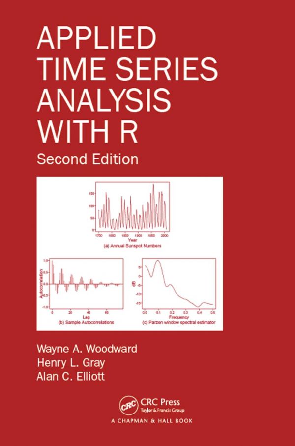
Applied Time Series Analysis with R
Virtually any random process developing chronologically can be viewed as a time series. In economics closing prices of stocks, the cost of money, the jobless rate, and retail sales are just a few examples of many. Developed from course notes and extensively classroom-tested, Applied Time Series Analysis with R, Second Edition includes examples across a variety of fields, develops theory, and provides an R-based software package to aid in addressing time series problems in a broad spectrum of fields. The material is organized in an optimal format for graduate students in statistics as well as in the natural and social sciences to learn to use and understand the tools of applied time series analysis. Features Gives readers the ability to actually solve significant real-world problems Addresses many types of nonstationary time series and cutting-edge methodologies Promotes understanding of the data and associated models rather than viewing it as the output of a “black box” Provides the R package tswge available on CRAN which contains functions and over 100 real and simulated data sets to accompany the book. Extensive help regarding the use of tswge functions is provided in appendices and on an associated website. Over 150 exercises and extensive support for instructors The second edition includes additional real-data examples, uses R-based code that helps students easily analyze data, generate realizations from models, and explore the associated characteristics. It also adds discussion of new advances in the analysis of long memory data and data with time-varying frequencies (TVF).

Applied Time Series Analysis with R 2nd Table of contents:

1: Stationary Time Series
1.1 Time Series
1.2 Stationary Time Series
1.3 Autocovariance and Autocorrelation Functions for Stationary Time Series
1.4 Estimation of the Mean, Autocovariance, and Autocorrelation for Stationary Time Series
1.4.1 Estimation of µ
1.4.1.1 Ergodicity of X
1.4.1.2 Variance of X
1.4.2 Estimation of γk
1.4.3 Estimation of ρk
1.5 Power Spectrum
1.6 Estimating the Power Spectrum and Spectral Density for Discrete Time Series
1.7 Time Series Examples
1.7.1 Simulated Data
1.7.2 Real Data
Appendix 1A: Fourier Series
Appendix 1B: R Commands
Exercises
2: Linear Filters
2.1 Introduction to Linear Filters
2.1.1 Relationship between the Spectra of the Input and Output of a Linear Filter
2.2 Stationary General Linear Processes
2.2.1 Spectrum and Spectral Density for a General Linear Process
2.3 Wold Decomposition Theorem
2.4 Filtering Applications
2.4.1 Butterworth Filters
Appendix 2A: Theorem Poofs
Appendix 2B: R Commands
2B.1 R Commands
Exercises
3: ARMA Time Series Models
3.1 MA Processes
3.1.1 MA(1) Model
3.1.2 MA(2) Model
3.2 AR Processes
3.2.1 Inverting the Operator
3.2.2 AR(1) Model
3.2.3 AR(p) Model for p ≥ 1
3.2.4 Autocorrelations of an AR(p) Model
3.2.5 Linear Difference Equations
3.2.6 Spectral Density of an AR(p) Model
3.2.7 AR(2) Model
3.2.7.1 Autocorrelations of an AR(2) Model
3.2.7.2 Spectral Density of an AR(2)
3.2.7.3 Stationary/Causal Region of an AR(2)
3.2.7.4 ψ-Weights of an AR(2) Model
3.2.8 Summary of AR(1) and AR(2) Behavior
3.2.9 AR(p) Model
3.2.10 AR(1) and AR(2) Building Blocks of an AR(p) Model
3.2.11 Factor Tables
3.2.12 Invertibility/Infinite-Order AR Processes
3.2.13 Two Reasons for Imposing Invertibility
3.3 ARMA Processes
3.3.1 Stationarity and Invertibility Conditions for an ARMA(p,q) Model
3.3.2 Spectral Density of an ARMA(p,q) Model
3.3.3 Factor Tables and ARMA(p,q) Models
3.3.4 Autocorrelations of an ARMA(p,q) Model
3.3.5 ψ-Weights of an ARMA(p,q)
3.3.6 Approximating ARMA(p,q) Processes Using High-Order AR(p) Models
3.4 Visualizing AR Components
3.5 Seasonal ARMA(p,q) × (PS,QS)S Models
3.6 Generating Realizations from ARMA(p,q) Processes
3.6.1 MA(q) Model
3.6.2 AR(2) Model
3.6.3 General Procedure
3.7 Transformations
3.7.1 Memoryless Transformations
3.7.2 AR Transformations
Appendix 3A: Proofs of Theorems
Appendix 3B: R Commands
Exercises
4: Other Stationary Time Series Models
4.1 Stationary Harmonic Models
4.1.1 Pure Harmonic Models
4.1.2 Harmonic Signal-Plus-Noise Models
4.1.3 ARMA Approximation to the Harmonic Signal-Plus-Noise Model
4.2 ARCH and GARCH Processes
4.2.1 ARCH Processes
4.2.1.1 The ARCH(1) Model
4.2.1.2 The ARCH(q0) Model
4.2.2 The GARCH(p0, q0) Process
4.2.3 AR Processes with ARCH or GARCH Noise
Appendix 4A: R Commands
Exercises
5: Nonstationary Time Series Models
5.1 Deterministic Signal-Plus-Noise Models
5.1.1 Trend-Component Models
5.1.2 Harmonic Component Models
5.2 ARIMA(p,d,q) and ARUMA(p,d,q) Processes
5.2.1 Extended Autocorrelations of an ARUMA(p,d,q) Process
5.2.2 Cyclical Models
5.3 Multiplicative Seasonal ARUMA (p,d,q) × (Ps, Ds, Qs)s Process
5.3.1 Factor Tables for Seasonal Models of the Form of Equation 5.17 with s = 4 and s = 12
5.4 Random Walk Models
5.4.1 Random Walk
5.4.2 Random Walk with Drift
5.5 G-Stationary Models for Data with Time-Varying Frequencies
Appendix 5A: R Commands
Exercises
6: Forecasting
6.1 Mean-Square Prediction Background
6.2 Box–Jenkins Forecasting for ARMA(p,q) Models
6.2.1 General Linear Process Form of the Best Forecast Equation
6.3 Properties of the Best Forecast Xto (l)
6.4 π-Weight Form of the Forecast Function
6.5 Forecasting Based on the Difference Equation
6.5.1 Difference Equation Form of the Best Forecast Equation
6.5.2 Basic Difference Equation Form for Calculating Forecasts from an ARMA(p,q) Model
6.6 Eventual Forecast Function
6.7 Assessing Forecast Performance
6.7.1 Probability Limits for Forecasts
6.7.2 Forecasting the Last k Values
6.8 Forecasts Using ARUMA(p,d,q) Models
6.9 Forecasts Using Multiplicative Seasonal ARUMA Models
6.10 Forecasts Based on Signal-Plus-Noise Models
Appendix 6A: Proof of Projection Theorem
Appendix 6B: Basic Forecasting Routines
Exercises
7: Parameter Estimation
7.1 Introduction
7.2 Preliminary Estimates
7.2.1 Preliminary Estimates for AR(p) Models
7.2.1.1 Yule–Walker Estimates
7.2.1.2 Least Squares Estimation
7.2.1.3 Burg Estimates
7.2.2 Preliminary Estimates for MA(q) Models
7.2.2.1 MM Estimation for an MA(q)
7.2.2.2 MA(q) Estimation Using the Innovations Algorithm
7.2.3 Preliminary Estimates for ARMA(p,q) Models
7.2.3.1 Extended Yule–Walker Estimates of the AR Parameters
7.2.3.2 Tsay–Tiao Estimates of the AR Parameters
7.2.3.3 Estimating the MA Parameters
7.3 ML Estimation of ARMA(p,q) Parameters
7.3.1 Conditional and Unconditional ML Estimation
7.3.2 ML Estimation Using the Innovations Algorithm
7.4 Backcasting and Estimating σ2a
7.5 Asymptotic Properties of Estimators
7.5.1 AR Case
7.5.1.1 Confidence Intervals: AR Case
7.5.2 ARMA(p,q) Case
7.5.2.1 Confidence Intervals for ARMA(p,q) Parameters
7.5.3 Asymptotic Comparisons of Estimators for an MA(1)
7.6 Estimation Examples Using Data
7.7 ARMA Spectral Estimation
7.8 ARUMA Spectral Estimation
Appendix
Exercises
8: Model Identification
8.1 Preliminary Check for White Noise
8.2 Model Identification for Stationary ARMA Models
8.2.1 Model Identification Based on AIC and Related Measures
8.3 Model Identification for Nonstationary ARUMA(p,d,q) Models
8.3.1 Including a Nonstationary Factor in the Model
8.3.2 Identifying Nonstationary Component(s) in a Model
8.3.3 Decision Between a Stationary or a Nonstationary Model
8.3.4 Deriving a Final ARUMA Model
8.3.5 More on the Identification of Nonstationary Components
8.3.5.1 Including a Factor (1 – B)d in the Model
8.3.5.2 Testing for a Unit Root
8.3.5.3 Including a Seasonal Factor (1 – Bs) in the Model
Appendix 8A: Model Identification Based on Pattern Recognition
Appendix 8B: Model Identification Functions in tswge
Exercises
9: Model Building
9.1 Residual Analysis
9.1.1 Check Sample Autocorrelations of Residuals versus 95% Limit Lines
9.1.2 Ljung–Box Test
9.1.3 Other Tests for Randomness
9.1.4 Testing Residuals for Normality
9.2 Stationarity versus Nonstationarity
9.3 Signal-Plus-Noise versus Purely Autocorrelation-Driven Models
9.3.1 Cochrane–Orcutt and Other Methods
9.3.2 A Bootstrapping Approach
9.3.3 Other Methods for Trend Testing
9.4 Checking Realization Characteristics
9.5 Comprehensive Analysis of Time Series Data: A Summary
Appendix 9A: R Commands
Exercises
10: Vector-Valued (Multivariate) Time Series
10.1 Multivariate Time Series Basics
10.2 Stationary Multivariate Time Series
10.2.1 Estimating the Mean and Covariance for Stationary Multivariate Processes
10.2.1.1 Estimating µ
10.2.1.2 Estimating Γ(k)
10.3 Multivariate (Vector) ARMA Processes
10.3.1 Forecasting Using VAR(p) Models
10.3.2 Spectrum of a VAR(p) Model
10.3.3 Estimating the Coefficients of a VAR(p) Model
10.3.3.1 Yule–Walker Estimation
10.3.3.2 Least Squares and Conditional ML Estimation
10.3.3.3 Burg-Type Estimation
10.3.4 Calculating the Residuals and Estimating Γa
10.3.5 VAR(p) Spectral Density Estimation
10.3.6 Fitting a VAR(p) Model to Data
10.3.6.1 Model Selection
10.3.6.2 Estimating the Parameters
10.3.6.3 Testing the Residuals for White Noise
10.4 Nonstationary VARMA Processes
10.5 Testing for Association between Time Series
10.5.1 Testing for Independence of Two Stationary Time Series
10.5.2 Testing for Cointegration between Nonstationary Time Series
10.6 State-Space Models
10.6.1 State Equation
10.6.2 Observation Equation
10.6.3 Goals of State-Space Modeling
10.6.4 Kalman Filter
10.6.4.1 Prediction (Forecasting)
10.6.4.2 Filtering
10.6.4.3 Smoothing Using the Kalman Filter
10.6.4.4 h-Step Ahead Predictions
10.6.5 Kalman Filter and Missing Data
10.6.6 Parameter Estimation
10.6.7 Using State-Space Methods to Find Additive Components of a Univariate AR Realization
10.6.7.1 Revised State-Space Model
10.6.7.2 ψj Real
10.6.7.3 ψj Complex
Appendix 10A: Derivation of State-Space Results
Appendix 10B: Basic Kalman Filtering Routines
Exercises
11: Long-Memory Processes
11.1 Long Memory
11.2 Fractional Difference and FARMA Processes
11.3 Gegenbauer and GARMA Processes
11.3.1 Gegenbauer Polynomials
11.3.2 Gegenbauer Process
11.3.3 GARMA Process
11.4 k-Factor Gegenbauer and GARMA Processes
11.4.1 Calculating Autocovariances
11.4.2 Generating Realizations
11.5 Parameter Estimation and Model Identification
11.6 Forecasting Based on the k-Factor GARMA Model
11.7 Testing for Long Memory
11.7.1 Testing for Long Memory in the Fractional and FARMA Setting
11.7.2 Testing for Long Memory in the Gegenbauer Setting
11.8 Modeling Atmospheric CO2 Data Using Long-Memory Models
Appendix 11A: R Commands
Exercises
12: Wavelets
12.1 Shortcomings of Traditional Spectral Analysis for TVF Data
12.2 Window-Based Methods that Localize the “Spectrum” in Time
12.2.1 Gabor Spectrogram
12.2.2 Wigner–Ville Spectrum
12.3 Wavelet Analysis
12.3.1 Fourier Series Background
12.3.2 Wavelet Analysis Introduction
12.3.3 Fundamental Wavelet Approximation Result
12.3.4 Discrete Wavelet Transform for Data Sets of Finite Length
12.3.5 Pyramid Algorithm
12.3.6 Multiresolution Analysis
12.3.7 Wavelet Shrinkage
12.3.8 Scalogram: Time-Scale Plot
12.3.9 Wavelet Packets
12.3.10 Two-Dimensional Wavelets
12.4 Concluding Remarks on Wavelets
Appendix 12A: Mathematical Preliminaries for This Chapter
Appendix 12B: Mathematical Preliminaries
Exercises
13: G-Stationary Processes
13.1 Generalized-Stationary Processes
13.1.1 General Strategy for Analyzing G-Stationary Processes
13.2 M-Stationary Processes
13.2.1 Continuous M-Stationary Process
13.2.2 Discrete M-Stationary Process
13.2.3 Discrete Euler(p) Model
13.2.4 Time Transformation and Sampling
13.3 G(λ)-Stationary Processes
13.3.1 Continuous G(p; λ) Model
13.3.2 Sampling the Continuous G(λ)-Stationary Processes
13.3.2.1 Equally Spaced Sampling from G(p; λ) Processes
13.3.3 Analyzing TVF Data Using the G(p; λ) Model
13.3.3.1 G(p; λ) Spectral Density
13.4 Linear Chirp Processes
13.4.1 Models for Generalized Linear Chirps
13.5 G-Filtering
13.6 Concluding Remarks 

People also search for Applied Time Series Analysis with R 2nd:

applied time series
    
penn state applied time series analysis
    
enders – applied time series
    
enders applied time series pdf
    
applied time series analysis pdf