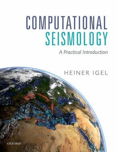
Computational Seismology A Practical Introduction 1st Edition by Heiner Igel ISBN 0191026859 9780191026850

Computational Seismology A Practical Introduction 1st Edition by Heiner Igel – Ebook PDF Instant Download/Delivery: 0191026859, 9780191026850
Full download Computational Seismology A Practical Introduction 1st Edition after payment

Product details:

ISBN 10: 0191026859 
ISBN 13: 9780191026850
Author: Heiner Igel

This book is an introductory text to a range of numerical methods used today to simulate time-dependent processes in Earth science, physics, engineering, and many other fields. The physical problem of elastic wave propagation in 1D serves as a model system with which the various numerical methods are introduced and compared. The theoretical background is presented with substantial graphical material supporting the concepts. The results can be reproduced with the supplementary electronic material provided as python codes embedded in Jupyter notebooks. The book starts with a primer on the physics of elastic wave propagation, and a chapter on the fundamentals of parallel programming, computational grids, mesh generation, and hardware models. The core of the book is the presentation of numerical solutions of the wave equation with six different methods: 1) the finite-difference method; 2) the pseudospectral method (Fourier and Chebyshev); 3) the linear finite-element method; 4) the spectral-element method; 5) the finite-volume method; and 6) the discontinuous Galerkin method. Each chapter contains comprehension questions, theoretical, and programming exercises. The book closes with a discussion of domains of application and criteria for the choice of a specific numerical method, and the presentation of current challenges.

Computational Seismology A Practical Introduction 1st Table of contents:

1 About Computational Seismology
1.1 What is computational seismology?
1.2 What is computational seismology good for?
1.3 Target audience and level
1.4 How to read this volume
1.5 Code snippets
Further reading
Part I Elastic Waves in the Earth
2 Seismic Waves and Sources
2.1 Elastic wave equations
2.2 Analytical solutions: scalar wave equation
2.3 Rheologies
2.3.1 Viscoelasticity and attenuation
2.3.2 Seismic anisotropy
2.3.3 Poroelasticity
2.4 Boundary and initial conditions
2.4.1 Initial conditions
2.4.2 Free surface and Lamb’s problem
2.4.3 Internal boundaries
2.4.4 Absorbing boundary conditions
2.5 Fundamental solutions
2.5.1 Body waves
2.5.2 Gradient, divergence, curl
2.5.3 Surface waves
2.6 Seismic sources
2.6.1 Forces and moments
2.6.2 Seismic wavefield of a double-couple point source
2.6.3 Superposition principle, finite sources
2.6.4 Reciprocity, time reversal
2.7 Scattering
2.8 Seismic wave problems as linear systems
2.9 Some final thoughts
Chapter summary
Further reading
Exercises
3 Waves in a Discrete World
3.1 Classification of partial differential equations
3.2 Strategies for computational wave propagation
3.3 Physical domains and computational meshes
3.3.1 Dimensionality: 1D, 2D, 2.5D, 3D
3.3.2 Computational meshes
3.3.3 Structured (regular) grids
3.3.4 Unstructured (irregular) grids
3.3.5 Other meshing concepts
3.4 The curse of mesh generation
3.5 Parallel computing
3.5.1 Physics and parallelism
3.5.2 Domain decomposition, partitioning
3.5.3 Hardware and software for parallel algorithms
3.5.4 Basic hardware architectures
3.5.5 Parallel programming
3.5.6 Parallel I/O, data formats, provenance
3.6 The impact of parallel computing on Earth Sciences
Chapter summary
Further reading
Exercises
Part II Numerical Methods
4 The Finite-Difference Method
4.1 History
4.2 The finite-difference method in a nutshell
4.3 Finite differences and Taylor series
4.3.1 Higher derivatives
4.3.2 High-order operators
4.4 Acoustic wave propagation in 1D
4.4.1 Stability
4.4.2 Numerical dispersion
4.4.3 Convergence
4.5 Acoustic wave propagation in 2D
4.5.1 Numerical anisotropy
4.5.2 Choosing the right simulation parameters
4.6 Elastic wave propagation in 1D
4.6.1 Displacement formulation
4.6.2 Velocity–stress formulation
4.6.3 Velocity–stress algorithm: example
4.6.4 Velocity–stress: dispersion
4.7 Elastic wave propagation in 2D
4.7.1 Grid staggering
4.7.2 Free-surface boundary condition
4.8 The road to 3D
4.8.1 High-order extrapolation schemes
4.8.2 Heterogeneous Earth models
4.8.3 Optimizing operators
4.8.4 Minimal, triangular, unstructured grids
4.8.5 Other coordinate systems
4.8.6 Concluding remarks
Chapter summary
Further reading
Exercises
5 The Pseudospectral Method
5.1 History
5.2 The pseudospectral method in a nutshell
5.3 Ingredients
5.3.1 Orthogonal functions, interpolation, derivative
5.3.2 Fourier series and transforms
5.4 The Fourier pseudospectral method
5.4.1 Acoustic waves in 1D
5.4.2 Stability, convergence, dispersion
5.4.3 Acoustic waves in 2D
5.4.4 Numerical anisotropy
5.4.5 Elastic waves in 1D
5.5 Infinite order finite differences
5.6 The Chebyshev pseudospectral method
5.6.1 Chebyshev polynomials
5.6.2 Chebyshev derivatives, differentiation matrices
5.6.3 Elastic waves in 1D
5.7 The road to 3D
Chapter summary
Further reading
Exercises
6 The Finite-Element Method
6.1 History
6.2 Finite elements in a nutshell
6.3 Static elasticity
6.3.1 Boundary conditions
6.3.2 Reference element, mapping, stiffness matrix
6.3.3 Simulation example
6.4 1D elastic wave equation
6.4.1 The system matrices
6.4.2 Simulation example
6.5 Shape functions in 1D
6.6 Shape functions in 2D
6.7 The road to 3D
Chapter summary
Further reading
Exercises
7 The Spectral-Element Method
7.1 History
7.2 Spectral elements in a nutshell
7.3 Weak form of the elastic equation
7.4 Getting down to the element level
7.4.1 Interpolation with Lagrange polynomials
7.4.2 Numerical integration
7.4.3 Derivatives of Lagrange polynomials
7.5 Global assembly and solution
7.6 Source input
7.7 The spectral-element method in action
7.7.1 Homogeneous example
7.7.2 Heterogeneous example
7.8 The road to 3D
Chapter summary
Further reading
Exercises
8 The Finite-Volume Method
8.1 History
8.2 Finite volumes in a nutshell
8.3 The finite-volume method via conservation laws
8.4 Scalar advection in 1D
8.5 Elastic waves in 1D
8.5.1 Homogeneous case
8.5.2 Heterogeneous case
8.5.3 The Riemann problem: heterogeneous case
8.6 Derivation via Gauss’s theorem
8.7 The road to 3D
Chapter summary
Further reading
Exercises
9 The Discontinuous Galerkin Method
9.1 History
9.2 The discontinuous Galerkin method in a nutshell
9.3 Scalar advection equation
9.3.1 Weak formulation
9.3.2 Elemental mass and stiffness matrices
9.3.3 The flux scheme
9.3.4 Scalar advection in action
9.4 Elastic waves in 1D
9.4.1 Fluxes in the elastic case
9.4.2 Simulation examples
9.5 The road to 3D
Chapter summary
Further reading
Exercises
Part III Applications
10 Applications in Earth Sciences
10.1 Geophysical exploration
10.2 Regional wave propagation
10.3 Global and planetary seismology
10.4 Strong ground motion and dynamic rupture
10.5 Seismic tomography—waveform inversion
10.6 Volcanology
10.7 Simulation of ambient noise
10.8 Elastic waves in random media
Chapter summary
Exercises
11 Current Challenges in Computational Seismology
11.1 Community solutions
11.2 Structured vs. unstructured: homogenization
11.3 Meshing
11.4 Nonlinear inversion, uncertainties
Appendix A Community Software and Platforms in Seismology
A.1 Wave propagation and inversion
A.2 Data processing, visualization, services
A.3 Benchmarking
A.4 Jupyter Notebooks
A.5 Supplementary material

People also search for Computational Seismology A Practical Introduction 1st:

computational seismology    
heiner igel computational seismology    
texas consortium for computational seismology    
computational seismology a practical introduction    
computational seismology book

Tags:

Heiner Igel,Computational,Seismology,practical Introduction