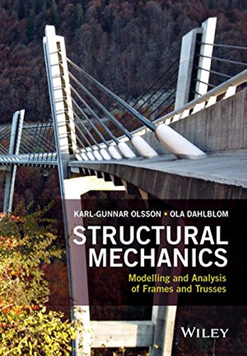
Structural Mechanics Modelling and Analysis of Frames and Trusses 1st Edition by Karl Gunnar Olsson, Ola Dahlblom 1119159360 9781119159360

Structural Mechanics : Modelling and Analysis of Frames and Trusses 1st Edition by Karl-Gunnar Olsson, Ola Dahlblom – Ebook PDF Instant Download/DeliveryISBN:  1119159360, 9781119159360 

Full download Structural Mechanics : Modelling and Analysis of Frames and Trusses 1st Edition after payment.

Product details:

ISBN-10 :  1119159360 

ISBN-13 :  9781119159360

Author:  Karl-Gunnar Olsson, Ola Dahlblom 

Textbook covers the fundamental theory of structural mechanics and the modelling and analysis of frame and truss structures

Structural Mechanics : Modelling and Analysis of Frames and Trusses 1st table of contents:

1 Matrix Algebra
1.1 Definitions
1.2 Addition and Subtraction
1.3 Multiplication
1.4 Determinant
1.5 Inverse Matrix
1.6 Counting Rules
1.7 Systems of Equations
1.7.1 Systems of Equations with Only Unknown Components in the Vector a
Example 1.1 Solving a system of equations with only unknown components in the vector a
1.7.2 Systems of Equations with Known and Unknown Components in the Vector a
Example 1.2 Solving a system of equations with both known and unknown components in the vector a
1.7.3 Eigenvalue Problems
Example 1.3 Solving an eigenvalue problem
Exercises
2 Systems of Connected Springs
Figure 2.1 Elastic spring and a system of connected springs
Figure 2.2 Nodes, degrees of freedom and connection of degrees of freedom
Figure 2.3 A spring element with two degrees of freedom
Figure 2.4 The quantities and relations of structural mechanics for springs and spring systems
2.1 Spring Relations
Figure 2.5 A spring with the stiffness k is loaded with the force N and thereby it is elongated by a distance δ
2.2 Spring Element
Figure 2.6 A discretised spring element
Figure 2.7 From spring to spring element
2.3 Systems of Springs
Figure 2.8 A system of connected springs
Figure 2.9 Global and local displacements
Figure 2.10 External forces at nodes
Figure 2.11 The free-body diagram of a spring element
Figure 2.12 Equilibrium for degree of freedom i
Figure 2.13 From element relations to system relations
Figure 2.14 Placement of the element stiffness matrix for element β into the global stiffness matrix according to the topology matrix in Equation (2.27)
Example 2.1 A system of springs
Figure 1 A system of three connected springs
Define a computational model
Figure 2 The computational model
Formulate element matrices
Compatibility conditions
Assemble element matrices
Define boundary conditions and loads
Solving the system of equations
Figure 3 Computed displacement
Figure 4 External equilibrium
Internal forces
Figure 5 Spring forces
Exercises
3 Bars and Trusses
Figure 3.1 An axially loaded bar and a two-dimensional (plane) truss
Figure 3.2 The quantities and relations of structural mechanics for bars and trusses
3.1 The Differential Equation for Bar Action
3.1.1 Definitions
Figure 3.3 From the material level to bar action
Figure 3.4 The principle for derivation of the constitutive relation of a higher level
Figure 3.5 The quantities of bar theory
3.1.2 The Material Level
Strain
Figure 3.6 System lines
Figure 3.7 Displacement and change in length (deformation) of a material fibre
Stress
Figure 3.8 The concept of stress
Figure 3.9 Linear elastic material relation
The Constitutive Relation of the Material
3.1.3 The Cross-Section Level
Kinematics
Figure 3.10 The displacement and the deformation du of the reference axis
Figure 3.11 Undeformed and deformed cross-section lamella
Force Relations
The Constitutive Relation at the Cross-Section Level
Figure 3.12 Normal stress and normal force
Figure 3.13 From the material level to the cross-section level
3.1.4 Bar Action
Kinematics
Equilibrium
Figure 3.14 Equilibrium for a slice of a bar
The Differential Equation for Bar Action
Figure 3.15 From cross-section level to bar action
3.2 Bar Element
3.2.1 Definitions
3.2.2 Solving the Differential Equation
Figure 3.16 From bar action to bar element
Figure 3.17 A bar element
Figure 3.18 The solution of the differential equation
Figure 3.19 A bar element in equilibrium
Figure 3.20 Axial load and equivalent element loads
Figure 3.21 From bar action to bar element
Example 3.1 A bar element with uniformly distributed load
Figure 1 A bar with uniformly distributed load
3.2.3 From Local to Global Coordinates
Figure 3.22 A bar element in a global coordinate system
Figure 3.23 Vector components
Figure 3.24 Direction cosines
Figure 3.25 Total vector action in the -direction
Figure 3.26 From local coordinates to global coordinates
3.3 Trusses
Figure 3.27 A truss and the associated computational model
Figure 3.28 From a bar element to a truss
Figure 3.29 The displacements of the bar element and the displacements of the truss
Figure 3.30 External forces that are introduced at the nodes in the computational model
Figure 3.31 A free-body diagram of a bar element
Figure 3.32 Equilibrium for degree of freedom i
Figure 3.33 From bar element to truss
Example 3.2 Truss
Figure 1 A plane truss consisting of three bars
Computational model
Figure 2 The computational model
Element matrices
Compatibility conditions
Assembling
Boundary conditions and nodal loads
Solving the system of equations
Figure 3 The computed displacements drawn in a magnified scale
Figure 4 The external load and the computed support forces
Compute internal forces
Figure 5 The normal forces in the bars
Exercises
4 Beams and Frames
Figure 4.1 Transversely loaded beam and a two-dimensional (plane) frame
Figure 4.2 The quantities and relations of structural mechanics for beams and frames
4.1 The Differential Equation for Beam Action
Figure 4.3 From the material level to beam action
4.1.1 Definitions
Figure 4.4 The quantities of beam theory
4.1.2 The Material Level
Strain
Stress
The Constitutive Relation of the Material
4.1.3 The Cross-Section Level
Kinematics
Figure 4.5 The deflection of the reference axis
Force Relations
Figure 4.6 Normal stress and bending moment
Figure 4.7 Shear stress and shear force
The Constitutive Relation at the Cross-Section Level
Figure 4.8 From the material level to the cross-section level
4.1.4 Beam Action
Kinematics
Equilibrium
Figure 4.9 Equilibrium for a small part of a beam
The differential equation for beam action
Figure 4.10 From the cross-section level to beam action
4.2 Beam Element
Figure 4.11 From beam action to a beam element in local coordinates
4.2.1 Definitions
4.2.2 Solving the Differential Equation for Beam Action
Figure 4.12 A beam element with four degrees of freedom
Figure 4.13 The solution of the differential equation
Figure 4.14 A beam element in equilibrium
Figure 4.15 Transverse load and equivalent element loads
Figure 4.16 From beam action to beam element
Example 4.1 A beam element with a uniformly distributed load
Figure 1 A beam element with a uniformly distributed load
4.2.3 Beam Element with Six Degrees of Freedom
Figure 4.17 From bar and beam elements in local coordinates to a beam element with six degrees of freedom in global coordinates
Figure 4.18 A beam element with six degrees of freedom
4.2.4 From Local to Global Directions
Figure 4.19 A beam element in a global coordinate system
Figure 4.20 From local coordinates to global coordinates
4.3 Frames
Figure 4.21 A frame and the associated computational model
Figure 4.22 From beam element to frame
Figure 4.23 From beam element to frame
Example 4.2 Frame
Figure 1 Frame
Computational model
Figure 2 Computational model
Element matrices
Compatibility conditions
Assembling
Boundary conditions
Solving the system of equations
Figure 3 Computed nodal displacements (translations and rotations) drawn in an exaggerated scale
Figure 4 External load and computed support forces
Displacements and internal forces
Figure 5 Displacements drawn in an exaggerated scale
Figure 6 The normal force, shear force and moment distributions
Figure 7 The section forces at the end points of Element 3
Exercises
5 Modelling at the System Level
Figure 5.1 A computational model
5.1 Symmetry Properties
Figure 5.2 Material symmetries
Figure 5.3 Symmetry plane and symmetry line
Figure 5.4 Symmetric structure, symmetric and anti-symmetric load
Figure 5.5 Symmetric load gives a symmetric mode of action
Figure 5.6 Anti-symmetric load gives an anti-symmetric mode of action
Figure 5.7 An element at the symmetry line
Figure 5.8 A simply supported structure with the corresponding boundary conditions at the symmetry line
Figure 5.9 Division of an arbitrary load into a symmetric and an anti-symmetric part
5.2 The Structure and the System of Equations
Figure 5.10 The structure and the system of equations
5.2.1 The Deformations and Displacements of the System
Figure 5.11 The displacement of a material point and the displacement degrees of freedom of the system
Figure 5.12 Kinematic assumptions
Adding Displacement Degrees of Freedom
Figure 5.13 Nodes with different numbers of displacement degrees of freedom
Constraints
Figure 5.14 Constraints – translation of degrees of freedom
Figure 5.15 Kinematic and static equivalence in the common cross-section
Figure 5.16 Beam element before and after translation of degrees of freedom
Figure 5.17 Constraints introduced at the system level
Figure 5.18 Constraints – rotation of degrees of freedom, of a rigid line and of a rigid body
Example 5.1 Constraints – translation of degrees of freedom
Figure 1 Beam with discontinuous system line
Computational model
Figure 2 Original beam element and beam element with translated degrees of freedom
Establishment of element relation
Figure 3 Constraints and static equivalence
Prescribed Displacements
5.2.2 The Forces and Equilibria of the System
Figure 5.19 To each degree of freedom an internal equilibrium equation is associated
Figure 5.20 A node with two extra equilibrium equations
Figure 5.21 Equilibria at different levels
5.2.3 The Stiffness of the System
The Diagonal of the Stiffness Matrix
Figure 5.22 Local stiffness in the direction of degree of freedom i
Figure 5.23 By static condensation, all stiffnesses along an internal force path can be gathered to a total stiffness
The Determinant of the Stiffness Matrix
Figure 5.24 Unstable structures, detK = 0
Static Condensation
Figure 5.25 Examples of applications for static condensation
Example 5.2 Static condensation – substructure
Figure 1 Bar with varying cross-sectional area
Computational model
Figure 2 Computational model
System of equations
Static condensation
Example 5.3 Static condensation – equivalent spring stiffness
Figure 1 Console beam with point load
Computational model
Figure 2 Computational model
Systems of equations and static condensation
Example 5.4 Reduction of a degree of freedom for an elementary case
Figure 1 A beam element with four degrees of freedom and a beam element where degree of freedom ū4 has been condensed out.
Canonical Stiffness
Figure 5.26 Deformation mode and the corresponding proportional load case, f = λa
Unit Displacement
Figure 5.27 A frame deformed by a unit displacement in the direction of degree of freedom i and the forces necessary to obtain this unit displacement
Figure 5.28 Elementary cases for a beam element with four degrees of freedom
Figure 5.29 Elementary cases for a beam element with three degrees of freedom
Figure 5.30 Element loads for a beam element with four degrees of freedom
Figure 5.31 Element loads for a beam element with three degrees of freedom
5.3 Structural Design and Simplified Manual Calculations
5.3.1 Characterising Structures
Figure 5.32 A statically indeterminate system. With kα ≫ kβ, the major part of the load fi is carried by the left spring
5.3.2 Axial and Bending Stiffness
Figure 5.33 Axial and bending stiffness
Figure 5.34 The influence of the shape, length and mode of action on the stiffness
Figure 5.35 The roof truss of the church of St. Catherine’s monastery (ca. 500 A.D.) and the Polonceau truss
5.3.3 Reducing the Number of Degrees of Freedom
Example 5.5 Reducing systems of equations
Figure 1 A frame structure modelled with 24 degrees of freedom
Figure 2 The frame structure according to Figure 1 modelled with consideration taken to the symmetry. The number of degrees of freedom in the computational model has been reduced to 15
Figure 3 A computational model with neglected axial deformations (a) and the substituted boundary conditions (b).
5.3.4 Manual Calculation Using Elementary Cases
Example 5.6 Identifying stiffness and element load from elementary cases
Figure 1 A frame with load and the computational model
Figure 2 Unit displacements and identified elementary cases
Exercises
6 Flexible Supports
Figure 6.1 Flexible supports
6.1 Flexible Supports at Nodes
Figure 6.2 Discrete elastic springs
Figure 6.3 A beam on a flexible support
6.2 Foundation on Flexible Support
Figure 6.4 Foundation on flexible support
6.2.1 The Constitutive Relations of the Connection Point
Figure 6.5 From connection point to foundation
Figure 6.6 The stiffness of the connection point
Figure 6.7 The local coordinate system, degrees of freedom and associated stiffnesses of the contact surface
6.2.2 The Constitutive Relation of the Base Surface
Kinematics
Figure 6.8 The kinematics of the base surface
Force Relations
Figure 6.9 Resulting forces
Constitutive Relation
6.2.3 Constitutive Relation for the Support Point of the Structure
Figure 6.10 Moving the reference point using constraints
Kinematics
Force Relation
Element Relations in Local and Global Coordinate System
6.3 Bar with Axial Springs
Figure 6.11 A bar with axial springs along its longitudinal direction
6.3.1 The Differential Equation for Bar Action with Axial Springs
Figure 6.12 The quantities of the differential equation
Figure 6.13 Deformed bar element
Kinematics
Equilibrium
Figure 6.14 Equilibrium for a part of a bar
The Differential Equation for a Bar with Axial Springs
6.3.2 Bar Element
Figure 6.15 A bar element with axial springs
Solving the Differential Equation
Example 6.1 Choice of element length for a bar with axial springs
Figure 1 A bar with axial springs
Figure 2 Displacement
Figure 3 Normal force
6.4 Beam on Elastic Spring Foundation
6.4.1 The Differential Equation for Beam Action with Transverse Springs
Figure 6.16 The quantities of the differential equation
Kinematics
Figure 6.17 Deformed beam element
Equilibrium
Figure 6.18 Equilibrium for a small part of a beam
The Differential Equation for a Beam with Transverse Springs
6.4.2 Beam Element
Figure 6.19 A beam element with transverse springs
Solving the Differential Equation
Example 6.2 Choice of element length for a beam with transverse springs
Figure 1 A beam with a transverse flexible support
Figure 2 Displacement
Figure 3 Moment
Figure 4 Shear force
Exercises
7 Three-Dimensional Structures
Figure 7.1 Three-dimensional beam and three-dimensional frame
Figure 7.2 Modes of action for a three-dimensional beam element
Figure 7.3 A three-dimensional beam element
Figure 7.4 Different representations of positive rotation and positive torque
Figure 7.5 From the element relation to a three-dimensional structure.
7.1 Three-Dimensional Bar Element
Figure 7.6 Three-dimensional bar element with local and global degrees of freedom
7.2 Three-Dimensional Trusses
Example 7.1 Truss
Figure 1 A three-dimensional truss consisting of four bars
Computational model
Figure 2 Computational model
Element matrices
Compatibility conditions
Assembling
Boundary conditions and nodal loads
Solving the system of equations
Figure 3 External load and computed support forces
Internal forces
Figure 4 Normal forces in the bars
7.3 The Differential Equation for Torsional Action
Figure 7.7 From material to torsional action
7.3.1 Definitions
Figure 7.8 The quantities of torsional action
7.3.2 The Material Level
Strain
Figure 7.9 Angular deformation for two material fibres in the cross-section plane, initially perpendicular to each other
Figure 7.10 Stress components related to torsion
Stress
The Constitutive Relations of the Material
7.3.3 The Cross-Section Level
Figure 7.11 Linear elastic material relations in shear
Figure 7.12 St. Venant torsion and Vlasov torsion
Figure 7.13 Solid and closed thin-walled cross-sections (St. Venant torsion) and open thin-walled cross-sections (Vlasov torsion)
Kinematics
Figure 7.14 Circular cross-section – plane cross-sectional surfaces remain plane. I-shaped cross-section – the cross-sectional surface is deformed in the -direction (warping)
Figure 7.15 The rotation of the cross-section about the reference axis (twist angle) and change of twist angle
Figure 7.16 Shear stresses and torque
Force Relations
The Constitutive Relations of the Cross-Section
Figure 7.17 From the material level to the cross-section level
Table 7.1 The coefficient α for rectangular massive cross-sections with different height–width relations h/b
Figure 7.18 Equilibrium for a slice of a twisted beam
7.3.4 Torsional Action
Kinematics
Equilibrium
The Differential Equation for Torsional Action
Figure 7.19 From the cross-section level to twist action
7.4 Three-Dimensional Beam Element
Figure 7.20 Three-dimensional beam element
Figure 7.21 Element for pure torsional action
7.4.1 Element for Torsional Action
7.4.2 Beam Element with 12 Degrees of Freedom
7.4.3 From Local to Global Directions
Figure 7.22 From local coordinates to global coordinates
7.5 Three-Dimensional Frames
Example 7.2 Frame
Figure 1 Three-dimensional frame with three beams
Computational model
Figure 2 Computational model
Element matrices
Compatibility conditions and assembling
Boundary conditions and nodal loads
Solving the system of equations
Figure 3 External load and computed support forces
Internal forces
Figure 4 Section forces in the elements
Exercises

People also search for Structural Mechanics : Modelling and Analysis of Frames and Trusses 1st:

 
computational structural mechanics
 
advanced structural mechanics
 
comsol structural mechanics module
 
fundamentals of structural mechanics
 
introduction to structural mechanics pdf

Tags: Structural Mechanics, Modelling, Analysis, Frames, Karl Gunnar Olsson, Ola Dahlblom